Part 2: Iterative Refinement with SSA Algorithm
Continuation from Part 1: SSA Algorithm Initialization
Welcome back to the second part of our exploration into Unit Commitment and Economic Dispatch MATLAB Code using the SSA Algorithm. In this segment, we delve deeper into the iterative refinement process that propels the SSA Algorithm towards optimized solutions.
Iterative Optimization:
As we embark on the iterative journey of SSA optimization, we kick off with the calculation of constants, namely C1, C2, and C3. These constants play a pivotal role in determining the new position of the swarm as the optimization progresses. C1 is calculated based on the current iteration and the maximum iteration.
Dynamic Swarm Movement:
The SSA Algorithm introduces dynamic swarm movement by generating random numbers. If C3 is less than 0.5, the new position of the swarm is determined by adding C1 multiplied by C2 to the best position obtained from the initial state. On the other hand, if C3 is greater than 0.5, the new position is obtained by subtracting C1 multiplied by C2 from the food position.
This dynamic movement ensures that the swarm explores different positions, balancing between exploration and exploitation in the search space.
Verification and Fitness Evaluation:
Following the swarm’s dynamic adjustment, we put it through a verification process. The swarm undergoes checks for minimum and maximum downtime, minimum uptime, and load coverage. If successful, the swarm moves forward, and its fitness is calculated using the objective function. The fitness is then compared with the leader’s fitness, determining whether the current swarm becomes the new leader.
This iterative process continues, with the swarm’s fitness being compared with the leader’s fitness. If the fitness is lower, the swarm assumes the role of the leader. The algorithm repeats this process for a set number of iterations.

Adaptation Over Time:
After 15 iterations, the algorithm introduces a new function to adjust the position of follower swarms. The follower swarm’s position is updated based on a combination of the current swarm and the previous one. This adaptive mechanism ensures continued exploration of the solution space.
Leadership Transition:
As the iterations progress, the algorithm dynamically selects leaders among the swarms. The leader’s fitness and position are determined based on comparisons with the food fitness and position. This transition of leadership is crucial for the convergence of the algorithm towards an optimal solution.
Conclusion of Iterations:
Iteratively repeating the refinement process for the defined maximum iteration, the SSA Algorithm actively displays the best fitness values in the command window. This showcases the progress and optimization achieved by the algorithm. With this, the iterative part of the SSA optimization concludes, paving the way for the next phase: result analysis.
In next we will delve into the results obtained and analyze the impact of the SSA Algorithm on Unit Commitment and Economic Dispatch MATLAB Code.
Part 3: Analysis and Results of SSA Optimization
Continuation from Parts 1 and 2: Unveiling the Results
Greetings once again! This marks the third installment in our exploration of Unit Commitment and Economic Dispatch through the lens of the SSA Algorithm. Now that we’ve navigated through the initialization and iterative refinement, let’s dive into the exciting part — the analysis of results.
Result Calculation:
With the state values of each generation established for the entire 24-hour period, we shift our focus to the calculation of results. This phase begins by defining the optimization type, such as economic dispatch, and initializing variables for fuel cost, emission cost, and other crucial parameters.
Optimization Variables:
We delve into the heart of the economic dispatch optimization, initiating the calculation of fuel cost and emission cost for the 24 hours. These variables are pivotal in understanding the economic and environmental impact of power generation.
Economic Dispatch Computation:
The optimization process involves computing H and C, where H is influenced by the C factor for each generation. These values are integral in the economic dispatch calculation, determining the optimal power allocation for each unit.
Quadprog Magic:
Enter quadprog – a MATLAB function that performs quadratic programming. This function takes into account the values of H, C, load power demand, and other parameters to efficiently calculate the economic dispatch. The result is a set of power values for each unit over 24 hours, providing a clear picture of the power generation landscape.
Costs and Emission Accumulation:
As the SSA Algorithm optimizes the economic dispatch, we accumulate fuel costs and emission costs for each hour. These metrics are vital in assessing the financial and environmental aspects of the power generation process.
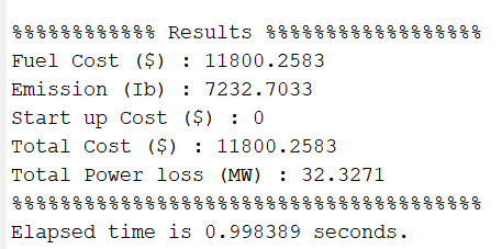
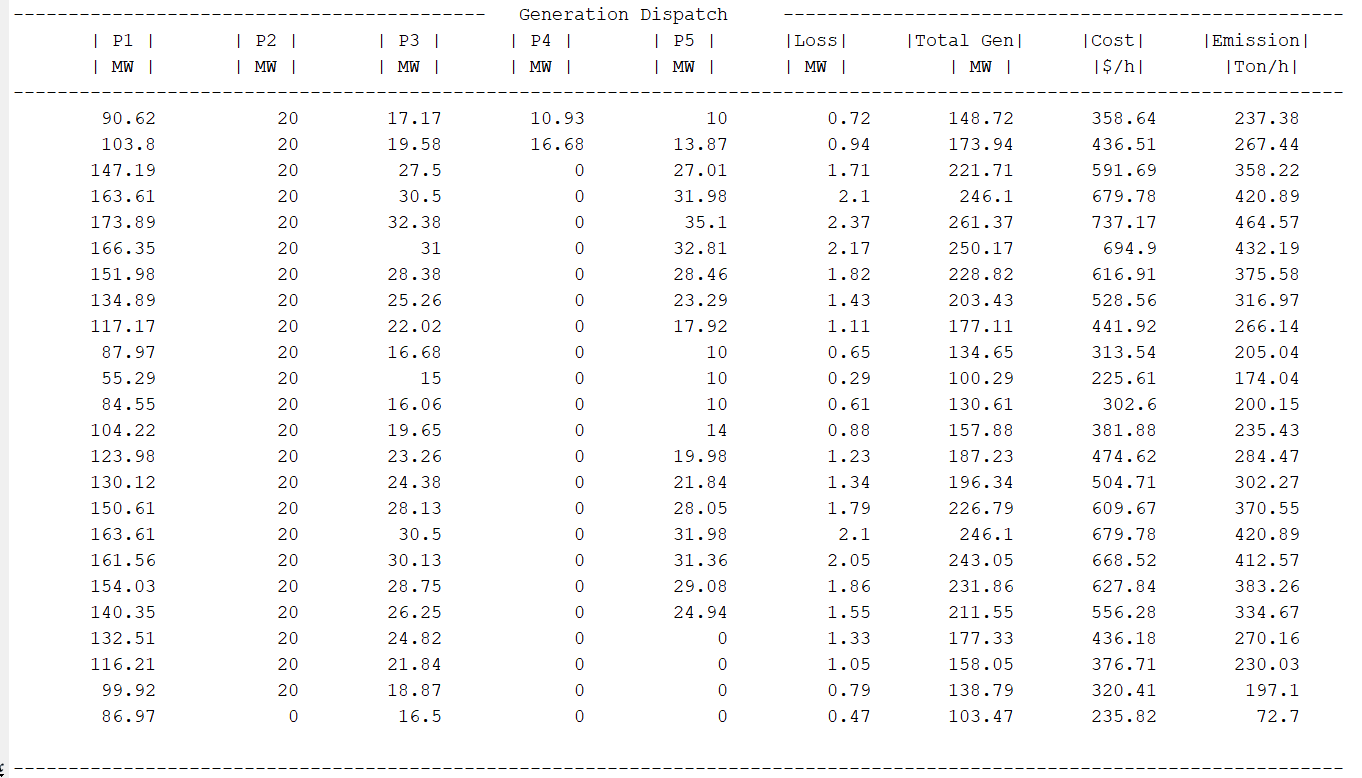
Visualizing the Outcome:
Bringing the results to life through visualizations, they are more than mere numbers. The display includes power output from each unit, power from wind, fuel costs, emission costs, startup costs, and the total cost for every hour of the 24 hours.
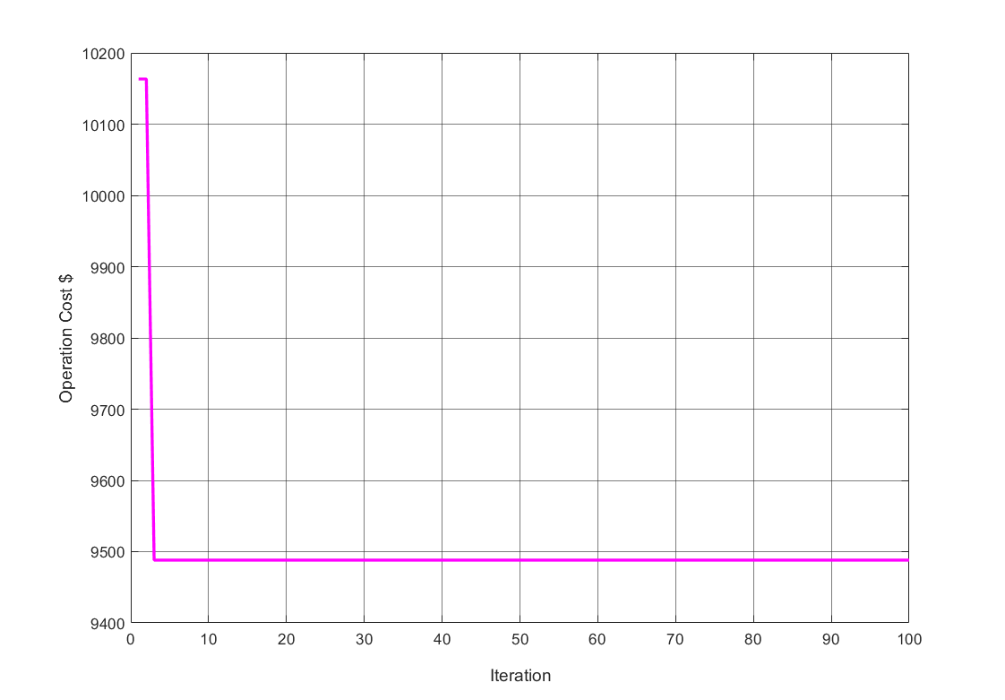
Plotting the Convergence Curve:
To gain deeper insights, we plot the convergence curve, illustrating how the optimization evolves over the iterations. This curve provides a visual representation of the algorithm’s convergence towards an optimal solution.
Hourly Breakdown:
Further breaking down the results, we create plots for each generation unit, showcasing their power output in each hour. Additionally, we visualize the cost and emission trends on an hourly basis.
Part 3 Conclusion:
As we wrap up the main function of the SSA Algorithm, we’ve witnessed the transformation of raw data into actionable insights. The optimization journey is complete, leaving us with a comprehensive understanding of how the SSA Algorithm enhances Unit Commitment and Economic Dispatch in MATLAB.
Stay tuned for the concluding part, where we’ll summarize the key takeaways and explore the implications of employing the SSA Algorithm in power system optimization. Until then, happy optimizing!
Part 4: Exploring Subfunctions and Program Logic
Continuation from Parts 1, 2, and 3: Unveiling the SSA Algorithm
Greetings once more! As we progress through our deep dive into Unit Commitment and Economic Dispatch using the SSA Algorithm, this segment sheds light on the subfunctions within the program and the underlying logic that drives the optimization process.
The Initial Function:
The program’s foundation lies in the “initial” subfunction. It begins by initializing the state variable ‘x’ for each generation over 24 hours. The randomness injected into this process ensures the exploration of a diverse solution space, contributing to the algorithm’s adaptability.
Verification Functions:
In enhancing the robustness of the SSA Algorithm, several verification functions are actively employed. These include the correction for minimum downtime, reserve constraint correction, and decommitment constraint correction. Each of these functions fine-tune the optimization process, addressing constraints and ensuring the feasibility of the generated solutions.
Object Function and Unit Commitment:
The crux of the SSA Algorithm is found in the “object” function, defining the unit commitment. SSA optimizes the state values ‘x’ for each generation, determining whether a unit should be on (1) or off (0). This unit commitment sets the stage for the subsequent economic dispatch calculation.
Economic Dispatch Calculation:
After establishing the unit commitment, the program actively delves into economic dispatch calculation using quadprog, considering various parameters such as maximum power, minimum power, power demand, and generation characteristics. This step ensures the optimal allocation of power resources.
Objective Function:
Bundling fuel costs, emission costs, and startup costs into the objective function, appropriately named “F object,” actively integrates these factors. This function quantifies the overall cost associated with power generation over the 24 hours. The SSA Algorithm aims to minimize this objective function, driving towards an optimal solution that balances economic and environmental considerations.
Understanding the SSA Optimization Process:
Recapping the essence of SSA, it optimizes the swarm’s values (represented by ‘x’) to minimize startup costs, fuel costs, and emission costs collectively. The dynamic nature of the algorithm allows it to explore different states for each generation over 24 hours, striving to find the most cost-effective and environmentally friendly solution.