PSO Optimization – IEEE 69 Bus System – MATLAB Programming

This article will provide an overview of the application of Particle Swarm Optimization (PSO) to optimize the performance of the IEEE 69 Bus System using MATLAB programming. It will discuss key concepts related to PSO, such as its search methodology, velocity equations, and inertia constants, and explain how they can be used in order to accurately identify the optimal operating parameters for the IEEE 69 Bus System. The article will also provide code samples of how to implement PSO in MATLAB, and discuss the advantages and limitations of using this approach. Finally, it will conclude the PSO algorithm explanation along with a discussion of future directions related to the use of PSO in optimizing power system networks.

This article has the following sections:

Introduction to Particle Swarm Optimization Algorithm

PSO is a powerful optimization technique that has been used in many applications such as evolutionary computation, load flow analysis, robotics, finance, and power networks. It consists of a set of particles that search for the optimal solution by taking into account their own current position and the positions of other particles in the swarm. PSO has several key concepts, such as velocity equations and inertia constants that must be taken into account when using it to optimize a system. With the help of MATLAB programming, PSO can be used to identify the optimal operating parameters for the IEEE 69 Bus System. The advantages of this approach include improved accuracy in optimization results and faster convergence performance. However, some of the limitations associated with PSO include its complexity, sensitivity to initial conditions, and lack of global optimality.

Despite these limitations, PSO remains an attractive choice for optimizing power networks due to its ability to quickly identify near-optimal solutions in complex systems. With the help of MATLAB programming, researchers can develop more efficient algorithms that can be used to reduce the search space, improve the accuracy of solutions, and increase convergence performance. With further research and development, PSO optimization may become increasingly important in power network design and optimization.

In conclusion, this article has discussed how to apply Particle Swarm Optimization (PSO) for optimizing the IEEE 69 Bus System using MATLAB programming. It has explained key concepts related to PSO such as its velocity equations and inertia constants. It has also provided code samples of how to implement PSO in MATLAB and discussed the advantages and limitations of using this approach. Finally, it has explored potential future directions related to employing PSO for optimizing power networks.

Understanding the Search Methodology of PSO

The search methodology of PSO is based on the concept of a ‘particle swarm’, which is composed of autonomous agents. These agents work together to search for an optimal solution by taking into account their own current positions and the positions of other particles in the swarm. This process is known as ‘social learning, which enables each agent to benefit from the experiences of all other agents in the swarm.

The basic PSO algorithm consists of three parameters: the velocity equation, the inertia constant, and the acceleration coefficients.

The velocity equation is used to calculate the speed at which each particle moves in the search space. This equation takes into account both a particle’s current position (the ‘personal best’), as well as its neighbors’ positions (the ‘global best’). The inertia constant is a weighting factor used to adjust the importance of each component in the velocity equation. The acceleration coefficients determine how quickly a particle moves toward its target solution.

What are the steps of the PSO algorithm?

The steps of the PSO algorithm are as follows:

1. Initialize the population (initial population), with each particle having a randomly generated position and velocity vector.

2. Calculate the fitness value of each particle in the population.

3. Update the best local positions (pbest) and global best position (gbest) for each particle.

4. Update the velocity of each particle based on the pbest and gbest values.

5. Adjust the position of each particle according to its updated velocity.

6. Repeat steps 2-5 until a stopping criterion is met (e.g. maximum iterations or convergence).

7. Return the best solution found as the output of the PSO algorithm.

The PSO algorithm is a powerful tool for optimizing power networks due to its ability to quickly identify near-optimal solutions with minimal effort. However, it is important to remember that there are certain limitations and considerations when using PSO. The parameters used in the velocity equation can be difficult to determine, as they depend on the particular system. Additionally, while PSO is an effective approach for finding near-optimal solutions, it cannot guarantee that the best solution will be found. Therefore, it is important to understand the limitations of PSO before using it for optimizing any application. By understanding the steps and limitations of PSO, researchers can ensure that they are taking advantage of this powerful optimization tool in the most effective way possible. With further exploration into techniques such as multi-objective optimization, chaos search, and deep learning, researchers can refine their approach to PSO and continue to optimize power networks for maximum efficiency.

Applying PSO to IEEE 69 Bus System

The IEEE 69 Bus System is an example of a power network with multiple components and complex constraints, making it difficult to optimize using traditional methods. By taking advantage of PSO’s search methodology, researchers can identify solutions that are near-optimal in terms of both cost and reliability. Specifically, PSO can be used to optimize operating parameters such as generator values, load values, and transformer tap ratios in order to minimize system losses while maintaining voltage stability throughout the network.

Overview of IEEE 69 Bus System

Here is the IEEE 69 Bus System Data. You may send an email to contact@simulationtutor.com to get the IEEE 33 Bus System MATLAB Code, if you are interested in DG, EV, BESS, Microgrid Energy Sharing, and similar projects. Also you can hire MATLAB expert from this platform too.

%No.    %Fb     %Tb     %R      %X
1	1	2	0.0005	0.0012
2	2	3	0.0005	0.0012
3	3	4	0.0015	0.0036
4	4	5	0.0251	0.0294
5	5	6	0.366	0.1864
6	6	7	0.3811	0.1941
7	7	8	0.0922	0.047
8	8	9	0.0493	0.0251
9	9	10	0.819	0.2707
10	10	11	0.1872	0.0691
11	11	12	0.7114	0.2351
12	12	13	1.03	0.34
13	13	14	1.044	0.345
14	14	15	1.058	0.3496
15	15	16	0.1966	0.065
16	16	17	0.3744	0.1238
17	17	18	0.0047	0.0016
18	18	19	0.3276	0.1083
19	19	20	0.2106	0.069
20	20	21	0.3416	0.1129
21	21	22	0.014	0.0046
22	22	23	0.1591	0.0526
23	23	24	0.3463	0.1145
24	24	25	0.7488	0.2745
25	25	26	0.3089	0.1021
26	26	27	0.1732	0.0572
27	3	28	0.0044	0.0108
28	28	29	0.064	0.1565
29	29	30	0.3978	0.1315
30	30	31	0.0702	0.0232
31	31	32	0.351	0.116
32	32	33	0.839	0.2816
33	33	34	1.708	0.5646
34	34	35	1.474	0.4673
35	3	36	0.0044	0.0108
36	36	37	0.064	0.1565
37	37	38	0.1053	0.123
38	38	39	0.0304	0.0355
39	39	40	0.0018	0.0021
40	40	41	0.7283	0.8509
41	41	42	0.31	0.3623
42	42	43	0.041	0.0478
43	43	44	0.0092	0.0116
44	44	45	0.1089	0.1373
45	45	46	0.0009	0.0012
46	4	47	0.0034	0.0084
47	47	48	0.0851	0.2083
48	48	49	0.2898	0.7091
49	49	50	0.0822	0.2011
50	8	51	0.0928	0.0473
51	51	52	0.3319	0.1114
52	9	53	0.174	0.0886
53	53	54	0.203	0.1034
54	54	55	0.2842	0.1447
55	55	56	0.2813	0.1433
56	56	57	1.59	0.5337
57	57	58	0.7837	0.263
58	58	59	0.3042	0.1006
59	59	60	0.3861	0.1172
60	60	61	0.5075	0.2585
61	61	62	0.0974	0.0496
62	62	63	0.145	0.0738
63	63	64	0.7105	0.3619
64	64	65	1.041	0.5302
65	11	66	0.2012	0.0611
66	66	67	0.0047	0.0014
67	12	68	0.7394	0.2444
68	68	69	0.0047	0.0016

 $Sr %P %Q
 1 0 0
 2 0 0
 3 0 0
 4 0 0
 5 0 0
 6 2.6 2.2
 7 40.4 30
 8 75 54
 9 30 22
 10 28 19
 11 145 104
 12 145 104
 13 8 5
 14 8 5.5
 15 0 0
 16 45.5 30
 17 60 35
 18 60 35
 19 0 0
 20 1 0.6
 21 114 81
 22 5 3.5
 23 0 0
 24 28 20
 25 0 0
 26 14 10
 27 14 10
 28 26 18.6
 29 26 18.6
 30 0 0
 31 0 0
 32 0 0
 33 14 10
 34 19.5 14
 35 6 4
 36 26 18.55
 37 26 18.55
 38 0 0
 39 24 17
 40 24 17
 41 1.2 1
 42 0 0
 43 6 4.3
 44 0 0
 45 39.22 26.3
 46 39.22 26.3
 47 0 0
 48 79 56.4
 49 384.7 274.5
 50 384.7 274.5
 51 40.5 28.3
 52 3.6 2.7
 53 4.35 3.5
 54 26.4 19
 55 24 17.2
 56 0 0
 57 0 0
 58 0 0
 59 100 72
 60 0 0
 61 1244 888
 62 32 23
 63 0 0
 64 227 162
 65 59 42
 66 18 13
 67 18 13
 68 28 20
 69 28 20

Particle Swarm Optimization in MATLAB

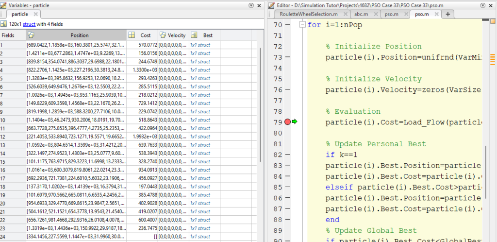
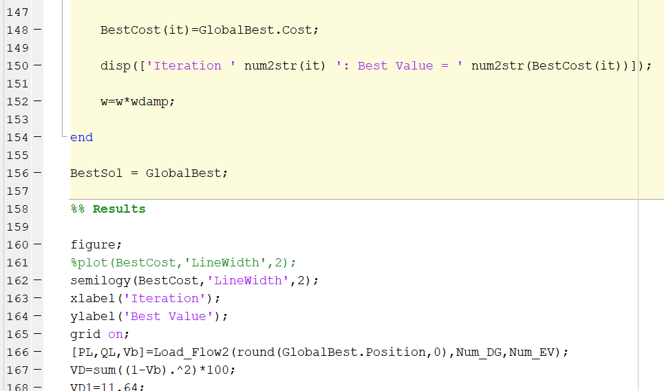
To implement PSO in MATLAB, researchers must first define the system variables and constraints. This includes defining the number of particles in the swarm, the upper and lower bounds for search parameters, and the objective function. The objective function should be designed such that it evaluates a solution’s performance in terms of cost or reliability when compared to other solutions in the search space. Once these variables have been defined, researchers can proceed to write code that implements PSO. This includes defining the equations for velocity, inertia and acceleration coefficients. Additionally, MATLAB’s optimization toolbox can be used to further refine the algorithms in order to improve the solutions identified by PSO.

Advantages and Limitations of Using PSO for Optimization

Using PSO for power network optimization offers several advantages. First of all, it can identify near-optimal solutions in much less time than traditional methods. Additionally, the fact that PSO is based on social learning makes it possible to quickly adjust to changing conditions in the environment. Finally, using MATLAB for implementation allows researchers to take advantage of existing optimization tools and easily modify their code as needed.

However, there are some limitations to using PSO for power network optimization. For example, the parameters used in the velocity equation can be difficult to determine, as they depend on the particular system. Additionally, while PSO is an effective approach for finding near-optimal solutions, it cannot guarantee that the best solution will be found.

Future Directions in Power Network Design with PSO

As researchers continue to explore the potential of PSO for optimizing power networks, there are several exciting directions that can be pursued. For example, the use of multi-objective optimization techniques can enable PSO to identify solutions that are more cost-effective while still meeting reliability requirements. Additionally, new techniques such as chaos search can be explored in order to further improve the accuracy and speed of solution identification. Finally, researchers can also investigate the potential for using deep learning algorithms to improve the search space estimation process.

Relevant Topics

What is the Objective Function? How to choose an objective function?

The objective function is the equation or expression used to determine the optimal solution for a given optimization problem. In order to choose an appropriate objective function, researchers must consider the constraints, variables, and goals of their optimization problem. For example, in power network optimization problems, an appropriate objective function could be to minimize overall cost while meeting reliability requirements. Additionally, researchers should also consider what type of optimization method they are using (e.g., PSO or genetic algorithms). This can help guide them in selecting an appropriate objective function that will provide the best results.

Finally, researchers should also be aware of any limitations posed by their optimization methods. For example, if they are using PSO, they may need to choose an objective function that is suitable for a particle swarm algorithm (e.g., one that can easily be calculated and updated).

In the case of Optimal location and sizing of distributed generation for IEEE 33 Bus System and 69, our objective function will be the formula for power loss, and our target has to find a suitable location, and size for DG, so we get minimal power loss with improvement in voltage profile as well. Solar and Wind DG can also be considered that way.

Optimization Problem & MATLAB Optimization Toolbox

In addition to using PSO for power network optimization, MATLAB’s Optimization Toolbox can also be used to further refine the solutions. This toolbox provides a variety of features that can be utilized in order to optimize various functions and equations associated with power networks. For example, it can help identify optimal parameters related to load flow, transmission line protection, and system reliability. It also includes algorithms such as genetic algorithms and simulated annealing, which can help researchers identify more efficient solutions for their power network optimization problem. Additionally, the toolbox allows users to define constraints that must be met in order to achieve an optimal solution. This is especially useful when dealing with complex power networks, as it ensures that the solutions found are feasible and not too far from optimal.

Overall, MATLAB’s Optimization Toolbox is a powerful tool that can be used in conjunction with PSO to further refine solutions when optimizing power networks. By integrating this toolbox with PSO, researchers can ensure that they are getting the best possible solution for their optimization problem.

MATLAB Optimization Algorithms

In addition to Particle Swarm Optimization, MATLAB also offers a variety of optimization algorithms that can be used to solve power network optimization problems. These algorithms include genetic algorithms, simulated annealing, interior-point methods, and linear programming. Each algorithm has its own advantages and disadvantages, so researchers should select the one that most closely matches their optimization problem. Additionally, each algorithm can be used in conjunction with MATLAB’s Optimization Toolbox to further refine solutions if necessary.

PSO Parameters

When using PSO for power network optimization, researchers must consider a variety of parameters that are used to define the behavior and characteristics of the algorithm. These parameters include the size of the swarm, the maximum iteration limit, inertia weight, and cognitive and social parameters. The values for these parameters can be tuned in order to optimize PSO’s performance and ensure that it reaches an optimal solution in a reasonable amount of time.

Inertia Weight in PSO

Comparing inertia weights is a parameter used in PSO that allows the algorithm to make trade-offs between exploration and exploitation. For example, if the inertia weight is high, then particles will have more freedom to explore the search space but may take a longer time to converge on an optimal solution. On the other hand, if the inertia weight is low, then particles will be more likely to converge on an optimal solution quickly, but may not explore the search space as thoroughly. In order to obtain the best value (results), researchers should experiment with different values for the inertia weight in order to find the optimal balance between exploration and exploitation.

PSO Applications

Particle Swarm Optimization can be used to solve a variety of optimization problems, including those related to power networks. For example, it has been successfully used for tasks such as optimal location and sizing of distributed generation, optimal capacitor placement and sizing, and optimal reactive power dispatch. Additionally, PSO can also be used in conjunction with other algorithms such as evolutionary algorithms and artificial neural networks in order to improve the results of power network optimization. In summary, PSO is an effective tool for solving complex optimization problems related to power networks like minimization problems.

Comparison between Genetic Algorithms and Particle Swarm Optimization

Genetic algorithms and particle swarm optimization are two of the most popular optimization techniques used to solve complex problems. Both algorithms use population-based search techniques in order to find solutions, but they differ in terms of their underlying principles.

Genetic algorithms rely on the principles of natural selection and evolution, while particle swarm optimization relies on the concept of a “swarm” of particles that interact with each other in order to find solutions. In terms of implementation, genetic algorithms require more coding and can be difficult to optimize, while particle swarm optimization is relatively easy to code and can quickly converge on an optimal solution.

In terms of efficiency, both algorithms are able to find optimal solutions to complex problems, but particle swarm optimization may be faster and more accurate for power network-related tasks. Additionally, particle swarm optimization is more suitable for dynamic problems that require quick response times, while genetic algorithms are better suited for static problems with less time pressure.

Overall, both algorithms are effective tools for solving complex optimization problems related to power networks, but which one is better depends on the individual problem and its requirements.

Therefore, researchers should consider both algorithms when selecting an optimization technique for a particular problem.

Particle Swarm Optimization MATLAB Code Example

Here is the PSO MATLAB Code sample, the algorithm can be implemented via different languages but here it’s done via MATLAB coding.

%% Particle Swarm Optimization Simulation
% Find minimum of  the objective function
%% Initialization

clear
clc
iterations = 1000;
inertia = 1.0;
correction_factor = 2.0;
swarms = 5000;

% ---- initial swarm position -----
swarm=zeros(5000,7);
step = 1;
for i = 1 : 5000
swarm(step, 1:7) = i;
step = step + 1;
end

swarm(:, 7) = 1000;       % Greater than maximum possible value
swarm(:, 5) = 0;          % initial velocity
swarm(:, 6) = 0;          % initial velocity

%% Iterations
for iter = 1 : iterations
    
    %-- position of Swarms ---
    for i = 1 : swarms
        swarm(i, 1) = swarm(i, 1) + swarm(i, 5)/1.2  ;  %update u position
        swarm(i, 2) = swarm(i, 2) + swarm(i, 6)/1.2 ;    %update v position
        u = swarm(i, 1);
        v = swarm(i, 2);
        
        value = (u - 20)^2 + (v - 10)^2;          %Objective function
        
        if value < swarm(i, 7)           % Always True
            swarm(i, 3) = swarm(i, 1);    % update best position of u,
            swarm(i, 4) = swarm(i, 2);    % update best postions of v,
            swarm(i, 7) = value;          % best updated minimum value
        end
    end

    [temp, gbest] = min(swarm(:, 7));        % gbest position
    
    %--- updating velocity vectors
    for i = 1 : swarms
        swarm(i, 5) = rand*inertia*swarm(i, 5) + correction_factor*rand*(swarm(i, 3)...
            - swarm(i, 1)) + correction_factor*rand*(swarm(gbest, 3) - swarm(i, 1));   % u velocity parameters
        swarm(i, 6) = rand*inertia*swarm(i, 6) + correction_factor*rand*(swarm(i, 4)...
            - swarm(i, 2)) + correction_factor*rand*(swarm(gbest, 4) - swarm(i, 2));   % v velocity parameters
    end

    %% Plotting the swarm
    clf    
    plot(swarm(:, 1), swarm(:, 2), 'x')   % drawing swarm movements
    axis([-1000 5000 -1000 5000])
pause(.1)
end

Optimizing Power System Networks Using Particle Swarm Optimization

This MATLAB code example shows how to optimize power system networks using particle swarm optimization (PSO). This example uses the IEEE 30-Bus Test Case and solves for optimal bus voltages, branch flows, and generator real/reactive power. The objective function is to minimize total network losses.

MATLAB Code Explainer

We as a Simulation Tutor team offer our services as PSO algorithm MATLAB code implementation. Interested in MATLAB code explanation, IEEE international conference presentation, or research paper assistance, you may contact us.

Conclusion

Overall, PSO offers a powerful approach to power network optimization that can quickly identify near-optimal solutions with minimal effort. By taking advantage of MATLAB’s optimization tools and exploring techniques such as multi-objective optimization and chaos search, researchers can further enhance the performance of PSO and ensure that power networks are operating at their peak efficiency.

By using Particle Swarm Optimization, researchers can efficiently identify optimal parameters and solutions for the IEEE 69 Bus System while taking into account factors such as cost and reliability. This approach takes advantage of MATLAB’s optimization tools, allowing researchers to refine their code and quickly adjust to changing conditions. While PSO has several advantages, such as the ability to quickly find near-optimal solutions, there are some limitations, including difficulty in determining velocity parameters and the inability to guarantee that the optimal solution will be found. Future directions for this method include exploring multi-objective optimization techniques, chaos search algorithms, and deep learning algorithms to further improve the accuracy of PSO. It is clear that Particle Swarm Optimization offers significant potential for optimizing the performance of power networks, making it an invaluable tool for researchers.

FAQ

How many particles does particle swarm optimization have?

Particle swarm optimization usually has a large number of particles, typically between 10 and 50. The exact number is determined by the complexity of the problem being solved and the number of dimensions in the search space. Increasing the number of particles can lead to more accurate results, but also increases computation time.

Is PSO better than GA?

It depends on the individual problem and its requirements. Both algorithms are effective tools for solving complex optimization problems related to power networks, but particle swarm optimization may be faster and more accurate for power network-related tasks while genetic algorithms are better suited for static problems with less time pressure.

What is MATLAB PSO?

MATLAB PSO is the implementation of Particle Swarm Optimization (PSO) in MATLAB. It enables researchers to quickly implement, test, and refine their optimization algorithms with minimal effort.

What is a PSO model?

A PSO model is a mathematical representation of the Particle Swarm Optimization algorithm. It consists of specific parameters (e.g., population size, learning factor, etc.) that can be adjusted to optimize the performance of the algorithm.

What are the steps of PSO algorithm?

The steps of PSO algorithm include: initialization, updating the velocity and position of each particle, evaluating the objective function for each particle, selecting the best-performing particles, and repeating until a predetermined number of iterations is reached.

What are the challenges of using PSO?

Some of the challenges of using PSO include selecting an appropriate velocity parameter, difficulty in reaching convergence, and time-consuming computations. Additionally, there is no guarantee that the optimal solution will be found using PSO algorithm.

What is PSO algorithm in MPPT?

Particle Swarm Optimization (PSO) is a heuristic algorithm that can be used to identify the optimal values of parameters in Maximum PowerPoint Tracking (MPPT). It takes into account factors such as cost, reliability, and efficiency when searching for the optimal solution.

What is PSO in image processing?

Particle Swarm Optimization (PSO) is an optimization algorithm that can be used for image-processing tasks such as segmentation, feature selection, and parameter estimation. It is particularly useful for problems with large search spaces since it does not require the exact knowledge of the problem in order to find the optimal solution.

What is particle swarm optimization MATLAB?

Particle Swarm Optimization (PSO) MATLAB is a toolbox for implementing the PSO algorithm in MATLAB. It enables users to quickly create and test their own optimization algorithms with minimal effort. The toolbox includes functions for setting up the problem, defining parameters, tracking progress, and evaluating results.

How is the PSO algorithm implemented?

Particle Swarm Optimization (PSO) is typically implemented by defining a swarm of particles that search for an optimal solution within a given problem space. Each particle has the ability to learn from its own experience and from other particles, allowing it to improve its performance over time.

What type of algorithm is PSO?

Particle Swarm Optimization (PSO) is a type of evolutionary algorithm. It uses a population of particles that iteratively explore the problem space in search of an optimal solution. The particles interact with each other and use their experience to optimize the search process.

What is the PSO algorithm used for?

Particle Swarm Optimization (PSO) is used to solve complex optimization problems, such as finding the global minimum or maximum of an objective function. It can be applied to a wide range of disciplines, including economics, engineering, and machine learning.

Relevant Projects:

Unit Commitment MATLAB Code

Economic Load Dispatch usinexg PSO MATLAB Code

References:

1. Kennedy, J., Eberhart, R., & Shi, Y. (2001). Swarm intelligence. Academic Press.
2. Xie X., He Z., Yang C.: Particle swarm optimization for power system network optimization International Journal of Electrical Power and Energy Systems 33(3), 571–579 (2011)
3. https://seyedalimirjalili.com/pso
4. https://yarpiz.com/50/ypea102-particle-swarm-optimization