Embark on a journey into the nuanced realm of Economic Dispatch and Demand Response in Microgrids through this MATLAB tutorial. Leveraging the amalgamation of Differential Algorithm (DA) and Particle Swarm Optimization (PSO), this tutorial, rooted in MATLAB code, demystifies complexities, making it accessible for both novices and seasoned practitioners alike.
1. File Structure:
The meticulous organization of the MATLAB code into five files ensures clarity and modularity. Each file serves a specific purpose in the optimization process, promoting an organized and comprehensible structure for users.
2. Loading Input Data:
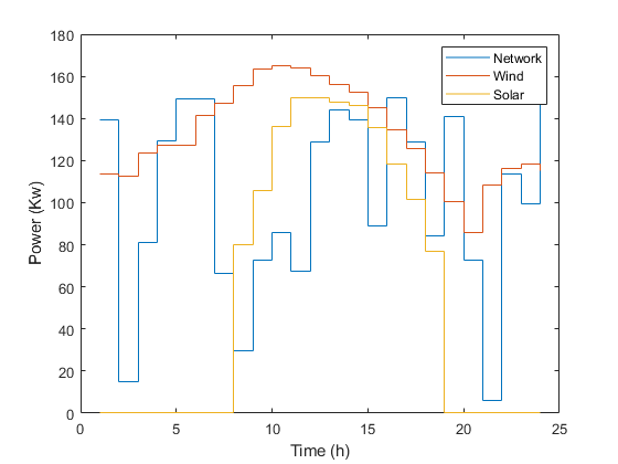
Initiating the process, the loading of input data encompasses vital solar and wind profiles. Decision variables are subsequently introduced, representing three generations, power from the network, and power demand response from three distinct customers. This initial step lays the groundwork for subsequent optimization.
3. Defining Constraints:
With decision variables in place, the next step involves defining constraints. Parameters such as minimum and maximum values, ramping upper and down ramps for each generation, and other critical elements are set. This ensures that the optimization adheres to practical operational limits, making the results more applicable to real-world scenarios.
4. Particle Swarm Optimization (PSO) Implementation
4.1 Initialization of PSO Parameters:
Central to the PSO algorithm is the initialization of key parameters. These include the number of iterations, population size, and velocity limits. A judicious setup of these parameters significantly influences the efficiency and effectiveness of the PSO algorithm.
4.2 Particle Initialization:
The uniform initialization of particle positions for 24 hours is a pivotal step. Subsequently, the load function is applied, imposing constraints to ensure that the load equals generation. This function also integrates wind and solar profiles while accommodating demand responses from customers.

43. PSO Main Loop:
The heart of the PSO algorithm lies in its main loop, which iterates over 600 cycles. Transitioning through each iteration, particles dynamically update positions based on velocity. To maintain feasibility, rigorously apply constraints, and evaluate the fitness function, which integrates economic dispatch and demand response, guiding particles toward optimal solutions.
4.4 Global Best Update:
Continuously refining, the global best position updates based on the minimum cost achieved across all particles. Simultaneously, individual particles update their personal best positions. This dynamic adjustment ensures a persistent search for improved solutions throughout the optimization process.
4.5. Results and Visualization:
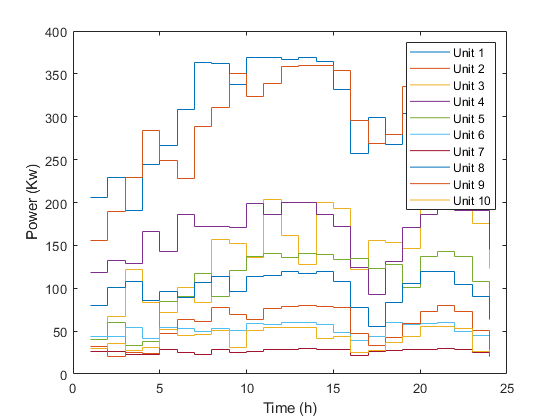
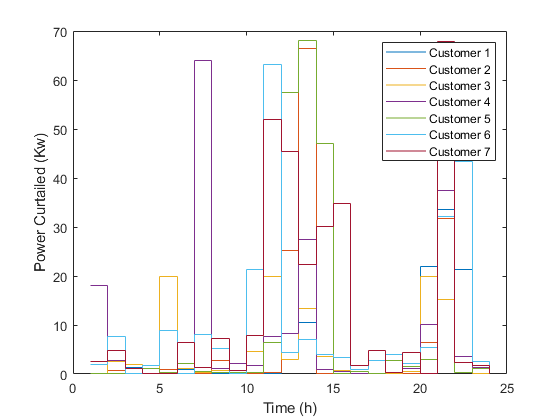
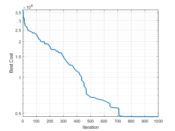
Upon the completion of iterations, the global best position is unveiled, showcasing the optimal solution for generation, network power, and customer responses. Through insightful plots, users gain a visual understanding of the cost evolution, power curtailed from customers, and power derived from various sources over time.

5. Dragonfly Algorithm (DA) for Economic Dispatch
5.1 Introduction to Dragonfly Algorithm:
Expanding the tutorial’s scope, an introduction to the Dragonfly Algorithm offers an alternate perspective on economic dispatch. Unique considerations specific to the Dragonfly Algorithm come to light, providing users with a comprehensive understanding of diverse optimization approaches.
5.2 DA Implementation:
Parallel to the PSO approach, the DA process involves the initialization of parameters, upper and lower limits, and iterative execution. The load function is applied, mirroring its role in PSO, ensuring adherence to load generation constraints and ramp rate constraints.

5.3 Fitness Function Evaluation:
A rigorous evaluation of the fitness function ensues, encompassing economic dispatch and demand response over 24 hours. Constraints are applied to customer incentives and energy curtailment, guaranteeing operational feasibility and refining the obtained solutions.
5.4 Results Display:
Results stemming from the DA algorithm are presented, emphasizing the optimal solutions achieved. Visual representations, through plots, offer insights into the cost evolution and power distribution over time, augmenting comprehension of the DA algorithm’s performance.
6. Case 2: Economic Dispatch and Demand Response
In this segment, we’ll delve into Case 2 of Economic Dispatch and Demand Response, building on the foundation laid in Case 1. While the overarching principles remain consistent, Case 2 introduces distinct data and initial parameters, providing a diverse perspective on microgrid optimization.
6.1 Input Data and Decision Variables:
The case begins by loading input data, including wind and solar profiles. Notably, the number of decision variables increases to 18, encompassing ten generators, one network connection, and seven customers. The decision variables, labeled P1 to P10 for generators, Pr for the network, and X1 to X7 for customers, set the stage for a more intricate optimization process.

6.2 Constraints and Initialization:
In the process of setting boundaries, it entails determining both minimum and maximum values for each variable and establishing upper and lower ramp rates for the ten generators. To adapt to the heightened complexity of decision variables, parameters, such as the maximum iteration (100) and population size (600), are adjusted accordingly. Consequently, this adjustment ensures a more refined and efficient optimization process. Initialization involves defining PSO parameters, and velocities, and initializing positions randomly.
6.3 Load Function Application:
Similar to Case 1, the load function is applied to ensure two key constraints: load equals generation minus demand response plus wind and solar profiles, and adherence to up and down ramp rates. This function plays a pivotal role in obtaining a new position that satisfies these constraints.
6.4 Fitness Function Calculation:
Evaluating the fitness function, which integrates economic dispatch and demand response, follows the same process as before. Initiating parameters for each generator and customer, the costs from conventional power and network are computed. Subsequently, the fitness function, which incorporates weight factors for customers, is applied to assess the total cost over 24 hours.
6.5 Constraint Application and Global Best Update:
Imposing constraints on customer incentive costs and the maximum energy curtailed, the global best cost is updated by comparing it with the best cost for each particle. If a particle’s cost is lower than the global best, both the global best position and cost are updated.

7. PSO Main Loop:
The main loop, spanning 1000 iterations in Case 2, iteratively refines solutions. Velocity updates, position adjustments, and constraint applications are repeated. The process ensures continuous improvement in the global best position and cost.
8. Results and Visualization:
9. Total Metrics Display:
Offering a comprehensive perspective on the microgrid’s performance, this overview meticulously delineates total conventional power costs, transferred power transaction costs, customer incentives, energy curtailed, conventional energy generated, and transferred energy.
Conclusion
In conclusion, this MATLAB tutorial is more than just a walkthrough; it is an immersive experience into Economic Dispatch and Demand Response in Microgrids. By integrating both PSO and DA algorithms, users gain a profound understanding of microgrid optimization, empowering them to apply these techniques adeptly in diverse real-world scenarios.
Case 2 enriches our understanding of Economic Dispatch and Demand Response in Microgrids, showcasing the adaptability of optimization algorithms to varying datasets and parameters. The intricate dance between decision variables, constraints, and algorithmic refinement highlights the power of MATLAB in addressing real-world energy challenges. For any queries or further clarification, feel free to connect with us.
Online MATLAB Tutoring
Are you eager to unlock the full potential of MATLAB for simulations and numerical analysis? Look no further! Simulation Tutor brings you a cutting-edge Online MATLAB Tutoring service tailored to your learning needs.
The End!
