I. Introduction
The Newton-Raphson method is a powerful algorithm used to solve many nonlinear equations. This method of solving equations involves iteratively finding the approximate solution for the equation by taking the derivative at each iteration and using that information to move toward a solution. In this tutorial, we will discuss how to use MATLAB code to implement the Newton-Raphson method.
A. Definition of the Newton-Raphson method
The Newton-Raphson method uses the concept of iterative approximation to find a solution to a nonlinear equation. Starting with an initial guess value for the solution, each iteration is used to refine that guess and move it closer to the actual solution. The iterations are based on linearization around the current guess by taking the derivative of the nonlinear equation at that point. The linear approximation is used to update the guess by subtracting the value of the linearization from the previous guess. This process is repeated until a solution is found.
B. Brief history of the method
The Newton-Raphson method was first proposed by Isaac Newton and Joseph Raphson in the late 17th century. It has since become a widely used method for solving nonlinear equations due to its rapid convergence and robustness. Over the years, it has been used to solve various engineering problems such as jet engine design, bridge design, and aircraft design. It is also used in finance and economics to calculate the present value of future cash flows.
C. Importance of the method in mathematics and engineering
The Newton-Raphson method is an important tool for mathematicians and engineers alike. It has enabled many breakthroughs in the fields of mathematics, engineering, and other scientific disciplines. For example, it has been used to solve a variety of differential equations which are essential for understanding physical phenomena such as fluid dynamics and thermodynamics. In addition, it is used to solve a variety of optimization problems in finance, economics, and engineering.
D. Overview of the MATLAB programming language
MATLAB is a popular programming language used by scientists and engineers to analyze data, create models, and solve equations. It is especially useful for numerical analysis and can be used to easily implement the Newton-Raphson method. MATLAB has powerful built-in ures that allow you to quickly solve equations with minimal coding effort.
II. Basic concepts
A. Basic concept of the Newton-Raphson method
Newton’s method is based on the idea of linearization around a current guess to update the guess and move it closer to the solution. The linear approximation is found by taking the derivative at that point and subtracting it from the previous guess. This process is repeated until a solution is found.
A. Function notation
Newton’s method is usually expressed using function notation. This notation consists of two parts: the function and its derivative. The function is written as f(x) where x represents the independent variable, and the derivative of the function is written as f’(x).
B. Derivative of a function
The derivative of a function is the rate of change of the function with respect to its independent variable. The derivative can be calculated using the formula d/dx f(x) = f’(x), where x is the independent variable and f’(x) is the first derivative of f with respect to x.
C. Newton’s method for approximating roots
The Newton-Raphson method can be used to find the roots, or solutions, of a function. To find the root of a function using Newton’s method, we need to start with an initial guess for the solution and then iteratively refine it using linear approximations. The iterations are repeated until the difference between the current guess and the actual solution is small enough that it can be considered a satisfactory approximation.
D. Stopping criteria
Newton’s method is an iterative process, so it is important to have stop criteria to determine when the algorithm has converged on a solution. The most common stopping criterion is the norm of the difference between the current guess and the actual solution being small enough that it can be considered a satisfactory approximation. Other criteria include maximum iterations and maximum error tolerance or tolerable error.
E. Convergence of the Newton-Raphson method
The Newton-Raphson method is a robust, reliable algorithm that usually converges very quickly on a solution. However, there are some cases in which the algorithm may fail to converge or take an excessively long time to do so. In such cases, it is important to be able to identify and diagnose the cause of the problem to avoid wasting time and effort. Common causes of non-convergence include poor initial guesses, ill-conditioned equations, and numerical roundoff errors.
III. Newton Raphson Method MATLAB Code Example
Newton’s method is a widely used root-finding algorithm that can be easily implemented in MATLAB, a powerful programming language for scientific computing and engineering. The method utilizes a combination of calculus, linear algebra, and numerical analysis to quickly converge on a solution. MATLAB’s built-in functions allow you to easily solve equations iterative process to approximate the roots of a function, starting with an initial guess and using the derivative of the function to improve the approximation at each step.
To use the Newton-Raphson method in the MATLAB program, one must first define the function and its derivative, and then create a function handle to pass to the method. The user then needs to provide an initial guess and specify the stopping criteria, and then the method can be run using a loop or MATLAB’s built-in function. The method can be used to find the roots of both linear and nonlinear functions. One of the advantages of using the Newton-Raphson method in MATLAB is that it is relatively fast and efficient, especially when compared to other root-finding methods. However, it is important to keep in mind that the method requires the derivative of the function to be defined, and in some cases, the method may not converge to the root.
A. Setting up the function and its derivative
The first step in using Newton’s method is to define the function and its derivative. The function is written as f(x) = 0, and the derivative is written as f’(x) = 0. The function handle for the function and its derivative can then be created and passed to the method.
B. Initial guess
Once the function and its derivative have been set up, an initial guess for the solution needs to be provided. This can either be a number or a vector depending on the dimension of the problem. The user needs to specify the stopping criteria for when the method should stop, such as a maximum number of iterations or a threshold for the norm of the difference between the current guess and the actual solution.
C. Iteration
Once the initial guess and stopping criteria have been specified, Newton’s method can be run using a loop or MATLAB’s built-in function. At each iteration, the derivative of the function is used to improve the approximation of the root. The algorithm continues until it has converged on a solution or the stopping criteria have been reached. The iterations can be monitored to check for any abnormalities, such as divergence from the true root or slow convergence.
D. Calculation of the function value and its derivative
At each iteration, the function value and its derivative must be calculated. The function value is used to compute the allowed error between the current approximation and the true root, and the derivative is used to update the approximation at each step. MATLAB provides several built-in features for calculating these values, such as the diff and fminbnd functions.
E. Update of the approximation
Finally, the approximation is updated using the derivative of the function. This can be done by subtracting the derivative from the current approximation (or alternatively, by adding the inverse of the derivative to the approximation). The new approximation is used in the next iteration until it has converged on a solution or the stopping criteria have been met.
F. Stopping criteria
The user needs to specify the stopping criteria in order for the method to determine when it should stop. This could be a maximum number of iterations, a threshold for the norm of the difference between the current guess and actual solution, or some other criteria. Once this has been determined, the method can be run until it has converged on the root or the stopping criteria have been reached.
G. Plotting the results
The results of Newton’s method can be plotted to visualize the convergence process. This can help identify any problems with the method, such as divergence or slow convergence, and can be used to adjust the parameters. MATLAB provides several features for plotting the results of the Newton-Raphson method, such as the plot and quiver functions.
IV. Advantages and limitations
The advantages of the Newton-Raphson method include:
- Speed: The method is relatively fast and efficient, especially when compared to other root-finding methods.
- Convergence: The method is known for its fast convergence, especially when an initial guess is close to the root.
- Flexibility: The method can be applied to both linear and nonlinear functions, making it a versatile tool for solving a wide range of problems.
- Local nature: The method is a local method, which means that it can converge to a root if the initial guess is sufficiently close to the root.
Limitations of the Newton-Raphson method include:
- Derivative requirement: The method requires the derivative of the function to be defined, which can be difficult or impossible to obtain in some cases.
- Convergence issues: The method may not converge to the root if the initial guess is far from the root or if the function has multiple roots or singularities.
- Sensitivity to the initial guess: The method can be sensitive to the initial guess, and a poor initial guess can lead to slow convergence or non-convergence.
- Linearity assumption: The method assumes that the function is well-behaved locally, which may not be the case for some nonlinear functions.
A. Comparison with other root-finding methods
- Fast Decoupled Load Flow (FDLF) method: This method is used to solve power flow problems in electrical power systems. It is a variant of Newton’s method, that uses an approximate Jacobian matrix to speed up the convergence. FDLF method is faster than Newton-Raphson, but it may not converge to the exact solution.
- Jacobi method: This method is an iterative method used to solve systems of linear equations. It is similar to the Gauss-Seidel method, but it uses the solution from the previous iteration to approximate the current solution. The Jacobi method is slower than Newton’s method, but it does not require the derivative of the function to be defined.
- Backward-Forward Sweep method: This method is used to solve power flow problems in electrical power systems. It is a variant of the Gauss-Seidel method that uses a forward-backward sweep to iteratively improve the solution. The Backward-Forward Sweep method is slower than the Newton-Raphson method, but it can handle non-linear systems of equations.
- Gauss-Seidel method: This method is an iterative method used to solve systems of linear equations. It uses the solution from the previous iteration to approximate the current solution. The Gauss-Seidel method is slower than the Newton-Raphson method, but it does not require the derivative of the function to be defined.
In summary, the Newton-Raphson method can be faster than other methods such as Jacobi, Gauss-Seidel, Backward-Forward Sweep, and FDLF but it requires the derivative of the function to be defined. While other methods like Jacobi, Gauss-Seidel, Backward-Forward Sweep, and FDLF are slower than Newton’s method but they do not require the derivative of the function to be defined.

B. Conditions under which the method is most effective
The Newton-Raphson method is most effective when the function being solved is well-behaved and has a single root in the vicinity of the initial guess. This means that the function should be smooth and its derivative should not be zero at the root. Additionally, the method is more efficient when the initial guess is close to the root, as it will converge faster. The method is also more efficient for solving non-linear equations than linear equations since it uses the derivative of the function to improve the approximation. However, the method may not converge or converge to a different root if the function has multiple roots or if the derivative is zero at the root. Therefore, it’s important to be mindful of the function’s behavior and the initial guess when using Newton’s method.
C. Possible problems and pitfalls
There are several possible problems and pitfalls that can arise when using the Newton-Raphson method. Some of these include:
- Non-convergence: The method may not converge to the root if the initial guess is far from the root or if the function has multiple roots or singularities.
- Convergence to a different root: The method may converge to a different root if the function has multiple roots or if the initial guess is not close enough to the desired root.
- Slow convergence: The method may converge slowly if the initial guess is far from the root or if the function is not well-behaved.
- Divergence: The method may diverge if the function has a singularity or if the derivative is zero at the root.
- Ill-conditioning: The method may be sensitive to the choice of initial guess and the accuracy of the derivative, and it is affected by the condition of the function’s Jacobian matrix.
- Local nature: The method is a local method, which means that it can converge to a root if the initial guess is sufficiently close to the root. However, if the initial guess is not close to the root, the method may not converge or converge to a different root.
To avoid these problems, it is important to carefully choose the initial guess and to be aware of the function’s behavior and the presence of multiple roots or singularities. It is also important to monitor the convergence of the method and to adjust the stopping criteria accordingly.

V. Examples
A. Simple example of finding a root of a quadratic equation
The equation to solve is x^2 – 4 = 0, which can be rearranged to x^2 = 4, so x = ± 2.
The Newton-Raphson method can be used to find the root of this equation, starting with an initial guess of x0 = 2.
The derivative of the function is 2x, and the equation can be rearranged as x1 = x0 – f(x0)/df(x0) = x0 – (x0^2 – 4)/(2x0) = x0/2 + 2/x0.
Newton’s method can be implemented in a for loop, with stopping criteria based on a tolerance level or a maximum number of iterations.
At each iteration, the new approximation x1 is calculated, and if the difference between x1 and x0 is below the tolerance, the loop is broken and the root is returned.
Here’s an example of how the Newton-Raphson method can be implemented in MATLAB to find the root of this quadratic equation using the mathematical formula
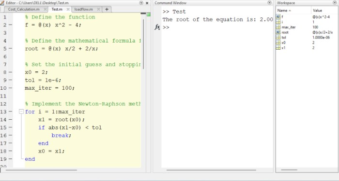
% Define the function and its derivative
f = @(x) x^2 - 4;
df = @(x) 2*x;

% Set the initial guess and stopping criteria
x0 = 2;
tol = 1e-6;
max_iter = 100;

% Implement the Newton-Raphson method
for i = 1:max_iter
    x1 = x0 - f(x0)/df(x0);
    if abs(x1-x0) < tol
        break;
    end
    x0 = x1;
end

% Print the root
root = x1;
fprintf("The root of the equation is: %f\n", root)
In this example, the Newton-Raphson method finds the root of the equation x^2 – 4 = 0, which is x = 2. The method is able to find the root using the mathematical formula for the root, which is x1 = x0/2 + 2/x0, and not by calculating the derivative of the function.
B. Newton Raphson Method for System of Nonlinear Equations MATLAB
Here’s an example of how to use Newton Raphson method for nonlinear systems of equations MATLAB example:
% Define the function and its derivative
f = @(x) exp(-x) - x;
df = @(x) -exp(-x) - 1;

% Set the initial guess and stopping criteria
x0 = 0.5;
tol = 1e-6;
max_iter = 100;

% Implement the Newton-Raphson method
for i = 1:max_iter
    x1 = x0 - f(x0)/df(x0);
    if abs(x1-x0) < tol
        break;
    end
    x0 = x1;
end

% Print the root
root = x1;
fprintf("The root of the equation is: %f\n", root)
In this example, the function is e^(-x) – x and its derivative is -e^(-x) – 1. The Newton-Raphson method is used to find the root of the function, starting with an initial guess of x0 = 0.5. The stopping criteria are set to a tolerance of 1e-6. The method will converge to the root of the function, which is approximately 0.567143, starting from the initial guess x0 = 0.5
In this example, the function is non-linear and Newton’s method is useful to find the root of the equation e^(-x) – x = 0. The Newton Raphson method is able to find the solution starting from a good initial guess and using the derivative of the function to improve the approximation at each step.
C. Load Flow Analysis by Newton Raphson Method using MATLAB
The Newton-Raphson method can also be applied to solve the load flow problem in power systems. The load flow problem is to find the voltage and current values at each bus in a power system network that satisfies the system’s power balance equations and voltage and current constraints. In power systems, the load flow problem is often formulated as a non-linear system of equations, and the Newton-Raphson method can be used to find the solution.
In MATLAB, the load flow problem can be formulated and solved using Newton’s method by defining the system’s equations, the Jacobian matrix, and the initial voltage and current values, then implementing the method in a for a loop until the solution converges. The solution obtained from the Newton-Raphson load flow can be used to analyze the power system’s stability and to design optimal control and protection schemes.
The example is the IEEE 14 bus system, Newton Raphson load flow MATLAB code and the equations to be solved are the power flow equations for the system.
clc,clear all,close all,
%% General Program For Newton Raphson Load flow
format short;
warning('off','all')
% Enter the busdata, and Loaddata in mention form
% Bus data (Bus	 Bus   Vol	   Vol	    Generating	  Load	   Reactive Power limit
%         	no   type  Mag(pu) angle PL     QL    Pg     Qg    Qmax   Qmin
busdata=  [ 1    1    1.06    0.0    0.0    0.0    0.0    0.0     0     0      0 %%in IEEE-13 bus system only 1 bus is slack here it is bus 1 other are PQ no PV bus is there
            2    2    1.04    0.0    0.0    0.0    0.0    0.0     0     0      0  %buses are 14 because with first bus I connect utility grid in etap so 14-1=13 bus which are as per 1EEE-13
            3    2    1.01    0.0    20     11.6   0.0    0.0     0     0      0
            4    3    1.00    0.0    17     12.5   0.0    0.0     0     0      0   %%column 5 is real power load and 6 is reactive power load
            5    3    1.00    0.0    23     13.2   0.0    0.0     0     0      0   %%column 7 is for real power gen and 8 is reactive power gen
            6    2    1.07    0.0    0.0    0.0    0.0    0.0     0     0      0
            7    3    1.00    0.0    40     29.0   0.0    0.0     0     0      0
            8    2    1.09    0.0    115.5  66.0   0.0    0.0     0     0      0
            9    3    1.00    0.0    0.00   0.00   0.0    0.0     0     0      0
            10   3    1.00    0.0    17.0   8.0    0.0    0.0     0     0      0.1
            11   3    1.00    0.0    12.8   8.6    0.0    0.0     0     0      0
            12   3    1.00    0.0    0.00   0.00   0.0    0.0     0     0      0
            13   3    1.00    0.0    17.0   15.1   0.0    0.0     0     0      0
            14   3    1.00    0.0    84.3   46.2   0.0    0.0     0     0      0.6];

%            From   To       R         X          B           Tap
%            Bus    Bus     (pu)      (pu)       (pu)         Ratio
%            From   To       R         X          B           Tap
%            Bus    Bus     (pu)      (pu)       (pu)         Ratio
linedata=    [1      2       0.01      0.08       0.00         1
              3      4       0.01759   0.05645    0.003451     1
              3      6       0.05601   0.07191    0.003111     1
              6      7       0.011     0.02       0.00         1
              4      5       0.01056   0.03389    0.002072     1
              2      3       0.07043   0.22600    0.0013818    1
              9      11      0.07384   0.06288    0.0073393    1
              3      8       0.07043   0.22600    0.013818     1
              8      9       0.03363   0.04317    0.0018681    1
              8      12      0.03520   0.11297    0.006907     1
              8      13      0.0001    0.00001    0.00         1
              9      10      0.03363   0.04317    0.0018681    1
             13      14      0.04610   0.03926    0.0045828    1];


%% Generation Input Data
% Initial Parameters
SPL=0;
VD=0;
Vb=zeros(14,1);
% N=length(DG)/3;
%%
Pg=zeros(14,1);
Qg=zeros(14,1);

%%

%% Bus data Bus type 1(slack Bus),type2(PV_Bus Bus), type3(PQ_Bus Bus)
tic
BMva=100;
% KV=11*10^3;
% Zbase=KV^2/BMva;
%% Data arranged for Linedata in the different vector
fb=linedata(:,1);tb=linedata(:,2);
r=linedata(:,3);x=linedata(:,4);
b=linedata(:,5);a=linedata(:,6);
z=(r+1i*x); 						% Impedance of branch
y=1./z;b=1i*b;  				% admittance of branch
nl=length(fb);					% No of branch
No_of_Bus=max(max(fb),max(tb));		% No of Bus

%% Formation of YBus matrix

Y=zeros(No_of_Bus,No_of_Bus);				% Initialize of YBus
for k=1:nl
    Y(fb(k),tb(k))=Y(fb(k),tb(k))-y(k)/a(k);
    Y(tb(k),fb(k))=Y(fb(k),tb(k));
end
for m=1:No_of_Bus
    for n=1:nl
        if fb(n)==m
            Y(m,m)=Y(m,m)+y(n)/a(n)^2+b(n);
        elseif tb(n)==m
            Y(m,m)=Y(m,m)+y(n)+b(n);
        end
    end
end
G=real(Y);B=imag(Y);			% Separation of YBus

Iter=1;Tol=1; % Iterantion And tolerance
%% Newton Raphson Load Flow
% Data arranged for Linedata in the different vector
busNo=busdata(:,1);V=busdata(:,3);del=busdata(:,4);
Pl=busdata(:,5)/BMva;       % it should be
Ql=busdata(:,6)/BMva;Qmin=busdata(:,9)/BMva;Qmax=busdata(:,10)/BMva;  %ql should be column 6
type=busdata(:,2);
Pg=(busdata(:,7)+Pg)/BMva;   %it should be column 7
Qg=(busdata(:,8)+Qg)/BMva;   %it should be coiumn 8
PV_Bus=find(type==2|type==1);PQ_Bus=find(type==3); % type1(Slack),type2(PV_Bus Bus),type3(PQ_Bus Bus )
No_of_PQ_Bus=length(PQ_Bus);No_of_PV_Bus=length(PV_Bus);
Active_Power_specified=Pg-Pl;Reactive_Power_specified=Qg-Ql; % Net Power flow through different node
%%%%%%%%%%%%%%%%%%%%%%%%%%%%%%%%%%%%%%%%%%%%%%%

while Tol>1e-5
    P=zeros(No_of_Bus,1);
    Q=zeros(No_of_Bus,1);
    for i=1:No_of_Bus
        for j=1:No_of_Bus
 P(i)=P(i)+V(i)*V(j)*(G(i,j)*cos(del(i)-del(j))+B(i,j)*sin(del(i)-del(j)));
 Q(i)=Q(i)+V(i)*V(j)*(G(i,j)*sin(del(i)-del(j))-B(i,j)*cos(del(i)-del(j)));
        end
    end
	% Verification of limit violation for reactive power
    if Iter>2 && Iter<=7
        for n=2:No_of_Bus
            if type(n)==2
                QG=Q(n)+Ql(n);
                if QG > Qmax(n)
                    V(n)=V(n)-0.01;
                elseif QG < Qmin(n)
                    V(n)=V(n)+0.01;
                end
            end
        end
    end
    dPa=Active_Power_specified-P;
    dQa=Reactive_Power_specified-Q;
    dP=dPa(2:No_of_Bus);
    k=1;
    dQ=zeros(No_of_PQ_Bus,1);
    for i=1:No_of_Bus
        if type(i)==3
            dQ(k,1)=dQa(i);
            k=k+1;
        end
    end
    M=[dP;dQ];% delta Matrix
	%% Formation Fo Jacobian Matrix[J1 J2;J3 J4]
	%% Formation Of J1
    J1=zeros(No_of_Bus-1,No_of_Bus-1);
    for i=1:No_of_Bus-1
        m=i+1;
        for j=1:No_of_Bus-1;
            n=j+1;
            if m==n
                for n=1:No_of_Bus
                J1(i,j)=J1(i,j)+V(m)*V(n)*(-G(m,n)*sin(del(m)-del(n))+B(m,n)*cos(del(m)-del(n)));
                end
                J1(i,j)=J1(i,j)-V(m)^2*B(m,m);
            else
                J1(i,j)=V(m)*V(n)*(G(m,n)*sin(del(m)-del(n))-B(m,n)*cos(del(m)-del(n)));
            end
        end
    end
	%% Formation Of J2
    J2=zeros(No_of_Bus-1,No_of_PQ_Bus);
    for i=1:No_of_Bus-1
        m=i+1;
        for j=1:No_of_PQ_Bus
            n=PQ_Bus(j);
            if m==n
                for n=1:No_of_Bus
                    J2(i,j)=J2(i,j)+V(n)*(G(m,n)*cos(del(m)-del(n))+B(m,n)*sin(del(m)-del(n)));
                end
                J2(i,j)=J2(i,j)+V(m)*G(m,m);
            else
                J2(i,j)=V(m)*(G(m,n)*cos(del(m)-del(n))+B(m,n)*sin(del(m)-del(n)));
            end
        end
    end
	%% Formation Of J3
    J3=zeros(No_of_PQ_Bus,No_of_Bus-1);
    for i=1:No_of_PQ_Bus
        m=PQ_Bus(i);
        for j=1:No_of_Bus-1
            n=j+1;
            if m==n
                for n=1:No_of_Bus
                    J3(i,j)=J3(i,j)+V(m)*V(n)*(G(m,n)*cos(del(m)-del(n))+B(m,n)*sin(del(m)-del(n)));
                end
                J3(i,j)=J3(i,j)-V(m)^2*G(m,m);
            else
                J3(i,j)=V(m)*V(n)*(-G(m,n)*cos(del(m)-del(n))-B(m,n)*sin(del(m)-del(n)));
            end
        end
    end
	%% Formation Of J4
    J4=zeros(No_of_PQ_Bus,No_of_PQ_Bus);
    for i=1:No_of_PQ_Bus
        m=PQ_Bus(i);
        for j=1:No_of_PQ_Bus
            n=PQ_Bus(j);
            if m==n
                for n=1:No_of_Bus
                J4(i,j)=J4(i,j)+V(n)*(G(m,n)*sin(del(m)-del(n))-B(m,n)*cos(del(m)-del(n)));
                end
                J4(i,j)=J4(i,j)-V(m)*B(m,m);
            else
                J4(i,j)=V(m)*(G(m,n)*sin(del(m)-del(n))-B(m,n)*cos(del(m)-del(n)));
            end
        end
    end
   J=[J1 J2;J3 J4]; % Jacobian Matrix
   X=inv(J)*M;
    dTh=X(1:No_of_Bus-1); % Change in angle
    dV=X(No_of_Bus:end);	% change in volatge mag
    del(2:No_of_Bus)=del(2:No_of_Bus)+dTh; % Voltage angle update
	% voltage mag update
    k=1;
    for n=2:No_of_Bus
        if type(n)==3
            V(n)=V(n)+dV(k);
            k=k+1;
        end
    end
    Iter=Iter+1;
    Tol=max(abs(M));
    if Iter>50
       Tol=0;
    else
    end
end
Q=zeros(No_of_Bus,1);
 for i=1:No_of_Bus
        for j=1:No_of_Bus
            P(i)=P(i)+V(i)*V(j)*(G(i,j)*cos(del(i)-del(j))+B(i,j)*sin(del(i)-del(j)));
            Q(i)=Q(i)+V(i)*V(j)*(G(i,j)*sin(del(i)-del(j))-B(i,j)*cos(del(i)-del(j)));
        end
 end
 for i=1:No_of_Bus
     del(i)=180*del(i)/pi; % Converion radian to degree
 end
 for i=1:14
Vb(i)=Vb(i)+V(i);
 end
 plot(Vb)
Vb
abs(P)
SPL=sum(abs(P))
QPL=sum(abs(Q))
Are you intrigued to discover more about how Newton Raphson MATLAB code can be used to enhance distributed generation and electric vehicle technology?
If you’d like to gain a deeper understanding, of MATLAB code for the Newton Raphson method click on the links provided!
Here Newton Raphson power flow MATLAB code is attached, and simulation is done which results in voltage profile, and real and reactive losses at each bus.
D. Jacobian Matrix – Newton Raphson method MATLAB – IEEE 14 Bus System
In an IEEE 14 bus system load flow program, the Jacobian matrix is used to approximate the local behavior of the system’s equations near a given point. The load flow problem in power systems is formulated as a non-linear system of equations, and Newton’s method is used to solve this system.
The Jacobian matrix is calculated as the matrix of partial derivatives of the vector-valued function F(x) with respect to the vector of variables x, where x represents the voltage and current values at each bus in the system. The elements of the Jacobian matrix are given by the partial derivatives of each equation of the system with respect to each variable.
The Jacobian matrix is calculated using the power flow equations which include the active and reactive power balance equations, the voltage magnitude constraints, and the current magnitude constraints. The Jacobian matrix is then used in the Newton-Raphson method to calculate the new approximation of the solution at each iteration.
In the IEEE 14 bus system load flow program, the Jacobian matrix is calculated by taking the partial derivatives of the power flow equations with respect to the voltage and current values at each bus. The resulting matrix is a sparse matrix that contains the sensitivity of the power flow equations to the voltage and current values. The Jacobian matrix is then used in the Newton-Raphson method, which is based on the idea of approximating the nonlinear function with a linear one around a current best approximation of the root, to calculate the new approximation of the solution at each iteration of the load flow calculation. The method uses Taylor’s Series representation of the function to calculate the new approximation of the root.
In summary, the Jacobian matrix is an important part of the load flow program in an IEEE 14 bus system, it is calculated by taking the partial derivatives of the power flow equations with respect to the voltage and current values at each bus, it is a sparse matrix that contains the sensitivity of the power flow equations to the voltage and current values, and it is used in Newton’s method to calculate the new approximation of the solution at each iteration.
Taylor’s series is a representation of a function as an infinite sum of terms, calculated using the function’s derivatives at a single point. The Taylor series of the cosine function can be represented as: cos(x) = 1 – (x^2)/2! + (x^4)/4! – (x^6)/6! + …
where x is the variable, and the exclamation mark denotes the factorial function. When the input value of x is large, the Taylor series can be truncated to a certain number of decimal places by calculating a limited number of terms. The resulting approximation of the function can be plotted as a figure output to visualize the difference between the original function and the approximation. This can be useful to understand the behavior of the function and the accuracy of the approximation. It is important to note that the Taylor series only provides an approximation of the function within a certain interval, and the error increases as x moves away from the interval. To learn more about the Taylor series and its application, one can ask question and look for answers in the mathematical literature.
In the Newton-Raphson method, the tangent line is used to approximate the behavior of the function near a given point. The tangent line is a linear function that has the same slope as the function at the given point, and it passes through the point. The Newton-Raphson method uses the tangent line to find the root of the function by finding the intersection of the tangent line with the x-axis.
The tangent line is calculated using the derivative of the function (Jacobian) and the current approximation of the root. The derivative of the function, also known as the slope, represents the rate of change of the function with respect to the variable, and it is used to calculate the slope of the tangent line. The current approximation of the root represents the point where the tangent line is drawn, and it is used to calculate the y-intercept of the tangent line.
The Newton-Raphson method requires the function to be differentiable at the point where the program is applied. It uses the derivative of the function (Jacobian) to calculate the tangent line which is used to approximate the behavior of the function. If the function is not differentiable or if the derivative is not well-defined, the approach may not converge or may converge to a wrong solution.
E. Newton Raphson Method MATLAB While Loop
The Newton-Raphson method in MATLAB can be implemented using a while loop. At each iteration of the loop, the Jacobian matrix and the vector of function values are used to calculate the new approximation of the solution. The while loop continues until the difference between two consecutive approximations is less than a predefined tolerance level or the maximum number of iterations is reached. In each iteration, the solution is updated with the new approximation and the loop will continue till the solution converges. This way, by using a while loop, the Newton-Raphson method MATLAB can find the root of the system of nonlinear equation efficiently. If you take a look at the code attached above, you’ll notice that MATLAB Newton Raphson code utilizes a while loop. This allows it to be much more efficient and effective than other solutions.
F. Newton Raphson MATLAB Function
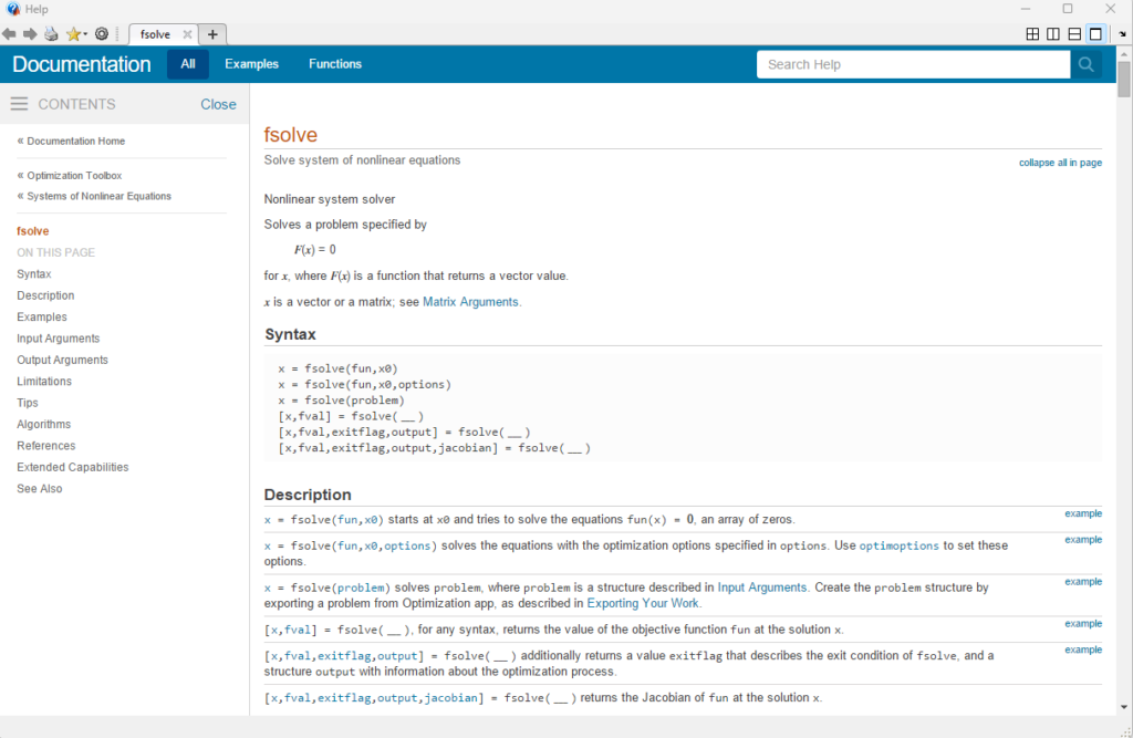
The fsolve function in MATLAB is a built-in function that can be used to solve systems of non-linear equations using the Newton-Raphson method. It is a convenient way to implement the Newton-Raphson method in MATLAB, as it automatically handles the iterative process and stopping criteria.
It can be used by passing the function and the initial guess as the input function, it will return the root of the equation. The fsolve function also allows users to specify the options for the solver, such as the tolerance level and the maximum number of iterations. The function uses the Jacobian matrix and the vector of function values to calculate the new approximation of the solution at each iteration and continues until the solution converges.
% Define the function to be solved
f = @(x) x^2 - 3;

% Define the initial guess
x0 = 1;

% Define the options for the solver
options = optimoptions('fsolve','Display','iter','TolFun',1e-6,'MaxIter',100);

% Use the fsolve function to solve the equation
root = fsolve(f,x0,options);

% Print the root
fprintf("The root of the equation is: %f\n", root)
In this example, the function to be solved is a simple equation x^2 -3, the initial guess is 1, and the options for the solver are set to display the iteration process, set the tolerance level to 1e-6, and the maximum number of iterations to 100. The fsolve function is then used to solve the equation and the returned solution is stored in the variable root. The final step is to print the root which is the solution of the equation.
The fsolve function uses the Newton-Raphson method, internally to finds the root of the function, by iteratively improving the approximation of the solution, until it converges to a predefined tolerance.
G. multivariable newton-Raphson method MATLAB
The Newton-Raphson method can also be used to find the roots of a system of non-linear equations with multiple variables. Here’s an example of Newton Raphson method for 2 variables MATLAB, non-linear equations:
Here is Newton Raphson’s multivariable MATLAB script (mfile):
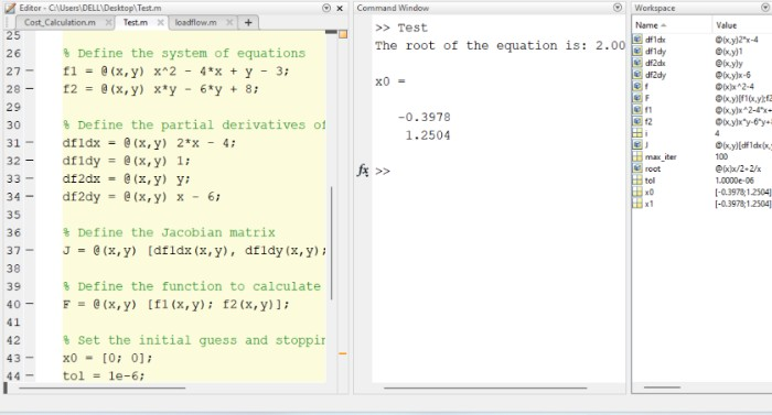
% Define the system of equations
f1 = @(x,y) x^2 - 4*x + y - 3;
f2 = @(x,y) x*y - 6*y + 8;

% Define the partial derivatives of the functions
df1dx = @(x,y) 2*x - 4;
df1dy = @(x,y) 1;
df2dx = @(x,y) y;
df2dy = @(x,y) x - 6;

% Define the Jacobian matrix
J = @(x,y) [df1dx(x,y), df1dy(x,y); df2dx(x,y), df2dy(x,y)];

% Define the function to calculate the F(x) vector
F = @(x,y) [f1(x,y); f2(x,y)];

% Set the initial guess and stopping criteria
x0 = [0; 0];
tol = 1e-6;
max_iter = 100;

% Implement the Newton-Raphson method
for i = 1:max_iter
    x1 = x0 - J(x0(1), x0(2))\F(x0(1), x0(2));
    if norm(x1-x0) < tol
        break;
    end
    x0 = x1;
end

% Print
H. Solving a Nonlinear Equation using Newton-Raphson Method
The Newton-Raphson method is a widely used program for solving nonlinear equations, which is based on the idea of approximating the nonlinear function with a linear one around a current best approximation of the root. The approach starts with an initial guess for the root and at each iteration, it uses the derivative of the function (Jacobian) to calculate a new approximation of the root by finding the root of the linearized function. The process continues until the difference between two consecutive approximations is less than a predefined tolerance or a maximum number of iterations is reached. The program is efficient and fast when the initial guess is close to the root.
The NR method can also be used to solve polynomial functions. A polynomial function can be written as the equation f(x) = a0 + a1x + a2x^2 + … + an*x^n
where a0, a1, a2, …, an are the coefficients of the polynomial and x is the variable. The Newton-Raphson method can find the root of a polynomial function by iteratively improving an approximation of the root, using the derivative of the function, which is also a polynomial function. The method is efficient and fast when the initial guess is close to the root. However, for some polynomials, the program may not converge, for example when the function has multiple roots or when the initial guess is far from the root. In these cases, other methods such as bisection, secant, or a combination of both can be used.
I. Modified Newton Raphson Method MATLAB Code
The Modified Newton-Raphson method is an extension of the standard Newton-Raphson approach that is used to find the roots of a system of non-linear equations with multiple variables. The method is implemented in MATLAB by first defining the system of equations, the partial derivatives of the functions, and the Jacobian matrix. Then, it uses the LU decomposition of the Jacobian matrix and the calculated L and U matrices to improve the approximation of the solution, which can prevent the method from diverging and converging faster.
The Modified Newton-Raphson program starts with an initial guess for the solution, and at each iteration, it uses the Jacobian matrix and LU decomposition to calculate the new approximation of the solution. The approach stops when the difference between two consecutive approximations is less than a predefined tolerance level or when the maximum number of iterations is reached. This modified method is useful when the Jacobian matrix is ill-conditioned and the standard Newton-Raphson program does not converge or converge slowly.
The MATLAB code provided below defines the system of equations, the partial derivatives of the example, the Jacobian matrix, and the F(x) vector. Then it performs LU decomposition of the Jacobian matrix and uses the resulting L and U matrices in the calculation of the new approximation x1. It also sets the initial guess and stopping criteria, implements the Modified Newton-Raphson method in a for loop, and prints the root of the system of equations when it’s found.
Here’s an example of how the Modified Newton-Raphson method can be implemented in MATLAB for a system of two non-linear equations with two variables:
% Define the system of equations
f1 = @(x,y) x^2 - 4*x + y - 3;
f2 = @(x,y) x*y - 6*y + 8;

% Define the partial derivatives of the functions
df1dx = @(x,y) 2*x - 4;
df1dy = @(x,y) 1;
df2dx = @(x,y) y;
df2dy = @(x,y) x - 6;

% Define the Jacobian matrix
J = @(x,y) [df1dx(x,y), df1dy(x,y); df2dx(x,y), df2dy(x,y)];

% Define the function to calculate the F(x) vector
F = @(x,y) [f1(x,y); f2(x,y)];

% Set the initial guess and stopping criteria
x0 = [0; 0];
tol = 1e-6;
max_iter = 100;

% Implement the Modified Newton-Raphson method
for i = 1:max_iter
    [L, U] = lu(J(x0(1), x0(2)));
    x1 = x0 - U\(L\F(x0(1), x0(2)));
    if norm(x1-x0) < tol
        break;
    end
    x0 = x1;
end

% Print the root
root = x1;
fprintf("The root of the system of equations is: [%f, %f]\n", root(1), root(2))
In this example, the Modified Newton-Raphson method is implemented by first performing LU decomposition on the Jacobian matrix and then using the resulting L and U matrices in the calculation of the new approximation x1. This program is useful when the Jacobian matrix is ill-conditioned and the standard Newton-Raphson method does not converge or converge slowly.
In this example, the Modified Newton-Raphson method is used to find the roots of a system of two non-linear equations with two variables x and y. The program uses the Jacobian matrix and LU decomposition to improve the approximation of the solution and it can converge to the root of the system of equations if the initial guess is close to the root and the Jacobian matrix is well-conditioned.
VI. Do my MATLAB Homework | Simulation Tutor
MATLAB is a powerful programming language for scientific computing and engineering, and it is commonly used in various fields such as engineering, physics, and mathematics. If you are struggling with your MATLAB homework, you may consider seeking help from a simulation tutor. A simulation tutor can guide you through the process of solving your homework problems and provide you with tips and techniques to help you understand the concepts better. They can also help you with debugging your code and provide feedback on your work.
They can also help you with more advanced topics such as image processing, machine learning, and optimization. Additionally, they can provide you with a good understanding of the software and how to use it effectively in your research or projects. They can also provide you with guidance on best practices and software design principles. By working with a simulation tutor, you can improve your understanding of the material and gain confidence in your ability to complete your homework assignments.

VII. Conclusion
In conclusion, the Modified Newton-Raphson method is a useful technique for finding the roots of a system of non-linear equations. It uses the Jacobian matrix and LU decomposition to improve the approximation of the solution, and it can converge to the root if the initial guess is close to the root and the Jacobian matrix is well-conditioned. Simulation tutors can be a great help when it comes to understanding and implementing this method in MATLAB. With their help, you can develop your understanding and skills in solving non-linear equations with MATLAB.
Moreover, simulation tutors can also help you with debugging your code and provide feedback on your work, as well as guidance on best practices and software design principles. With their help, you can improve your understanding of the material and gain confidence in your ability to complete your homework assignments.
By understanding the concept and properly implementing it in MATLAB, you can find the roots of a system of non-linear equations with the Modified Newton-Raphson approach.
A. Summary of key points
• The Modified Newton-Raphson method is a useful technique for finding the roots of a system of non-linear equations.
• It uses LU decomposition of the Jacobian matrix to improve the approximation of the solution.
• It can converge to the root if the initial guess is close to the root and the Jacobian matrix is well-conditioned.
• Simulation tutors can help with debugging code and provide feedback on work, as well as guidance on best practices and software design principles.
• By understanding the concept and properly implementing it in MATLAB, you can find the roots of a system of non-linear equations with the Modified Newton-Raphson method.
B. Future directions for research
There are several future directions for research on the Newton-Raphson approach and its variants:
Global Convergence: The Newton-Raphson program is known to converge quickly if the initial guess is close to the root, but it may not converge if the initial guess is far from the root. Research on methods that can ensure global convergence, such as combining the Newton-Raphson method with global optimization techniques, could be an area of future research.
High-dimensional systems: The Newton-Raphson approach can be applied to systems of non-linear equations with multiple variables, but the computational complexity increases with the number of variables. Research on methods that can efficiently solve high-dimensional systems, such as low-rank approximations or distributed computing, could be an area of future research.
Robustness to ill-conditioned Jacobians: The Newton-Raphson method can fail to converge if the Jacobian matrix is ill-conditioned, and the Modified Newton-Raphson method can resolve this problem. However, the Modified Newton-Raphson method may still fail when the Jacobian matrix is highly ill-conditioned. Research on methods that can improve the robustness of the Newton-Raphson method, such as regularization techniques, could be an area of future research.
Applications in machine learning: The Newton-Raphson method can be applied to optimize the parameters of machine learning models, such as neural networks. Research on methods that can improve the efficiency and scalability of the Newton-Raphson method for large-scale machine learning problems, such as stochastic gradient descent, could be an area of future research.
Hybrid methods: The Newton-Raphson method can be combined with other optimization methods to improve performance. Research on hybrid methods that combine the Newton-Raphson method with other optimization methods, such as Quasi-Newton or trust region methods, could be an area of future research.
C. Additional resources for further study
• The Newton-Raphson Method: Theory and Practice by H. Fendell (2002)
• Numerical Methods for Nonlinear Equations by R. Burden and J. Faires (2010)
• Numerical Optimization by J. Nocedal and S. Wright (2006)
VIII. References
- B. T. Polyak, “Introduction to Optimization,” New York: Optimization Software Inc., 1987.
- J. Nocedal and S. J. Wright, “Numerical Optimization,” New York: Springer, 2006.
- A. R. Conn, N. I. M. Gould, and P. L. Toint, “Trust Region Methods,” Philadelphia: SIAM, 2000.
- J. Nocedal and S. Wright, “Numerical Optimization,” 2nd ed. New York: Springer, 2006.
- R. Fletcher, “Practical Methods of Optimization,” 2nd ed. New York: John Wiley & Sons, 1987.
- K. Schittkowski, “Test Examples for Nonlinear Programming Codes,” Heidelberg: Springer, 1981.
- J. J. More, B. S. Garbow, and K. E. Hillstrom, “Testing Unconstrained Optimization Software,” ACM Trans. Math. Softw., vol. 7, pp. 17–41, 1981.